Standard

Index Laws

## \times = ##

## \div = ##

##\frac{{}}{{}} = ##

##{\left( {} \right)^b} = ##

##x^=\frac##

##x^=\frac##

a negative index means a fraction

##x^=\sqrt##

##x^=\sqrt[3]##

a fractional index means a root

Blood Alcohol Content – BAC

$$BA = \frac$$

N = number of drinks H = hours drinking M = Mass in kg

$$BA = \frac$$

Limitations on estimating BAC include food, medication interactions, errors in estimating the number of drinks and time period

$$t= \frac$$

time taken to reach a zero BAC

1 standard drink = 10 g alcohol

$$N = 0.789VA$$

N = number of standard drinks
V = volume of drink in L
A = alcohol percent content

Fried's Formula

Dosage for children 1 to 2 years = $$\frac$$

Young's Formula

Dosage for children 1 to 12 years = $$\frac$$

Clarke's Formula

Dosage = $$\frac$$

Distance, Speed and Time

$$d=st$$

$$s=\frac$$

$$t=\frac$$

Stopping Distance

Stopping Distance = Braking distance + Reaction time distance

Linear Modelling  – Straight Line

##y = mx + c##

where m is the gradient: $$m = \frac$$

c is the y-intercept

$$m=\frac$$

c is the y-intercept

to get x-intercept, set y = 0

to get y-intercept, set x = 0

Direct Variation

 $$y\,\ \propto\,x$$

$$y=kx$$

where k is the constant of variation

Pythagoras Theorem

c² = a² + b²

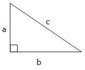
when looking for the hypotenuse

a² = c² – b²

when looking for a shorter side

a and b are the short sides c is the hypotenuse

Square

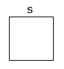
$$A=s^2$$

Rectangle

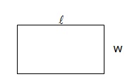
$$A=L\times\,w$$

Triangle

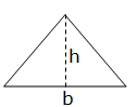
$$A=\frac\times \,b\times \,h$$

Triangle: Heron's Rule

$$A=\sqrt$$

$$s=\frac$$

where s is half the perimeter

Circle

$$A=\pi r^2$$

Annulus

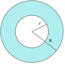
the annulus is the area between two circles, the 'donut'

$$A=\pi(R^2-r^2)$$

$$R=\sqrt$$

$$r=\sqrt$$

Trapezium

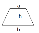
$$A=\frac(a+b)$$

Parallelogram

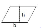
$$A=b\,\times\,h$$

Rhombus

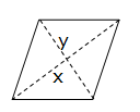
$$A=\frac\times\, x\times\,y$$

Kite

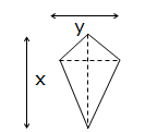
$$A=\frac\times\, x\times\, y$$

Cube

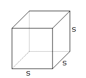
$$SA=6s^2$$

$$v=s^3$$

Rectangular Prism

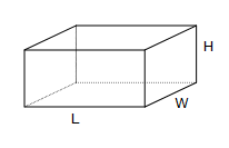
$$SA=2LW+2LH+2WH$$

$$V=LWH$$

Triangular Prism

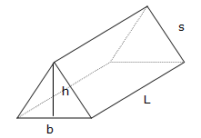
$$SA=2(\frac12bh)+2sL+bL$$

$$V=\frac12\, b hL$$

Pyramid

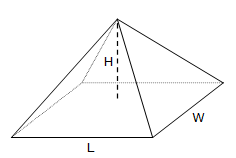
$$SA=LW+sum\,of \,triangles$$

$$V=\frac13\,LWH$$

Cylinder

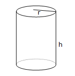
$$SA=2\pi \,r^2+2\pi \,rh$$

$$V=\pi \,r^2h$$

Cone

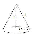
$$SA=\pi r^2+\pi\, rL$$

$$V=\frac13\pi \,r^2h$$

Sphere

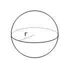
$$SA=4\pi \,r^2$$

$$V=\frac43\pi\, r^3$$

Arc Length

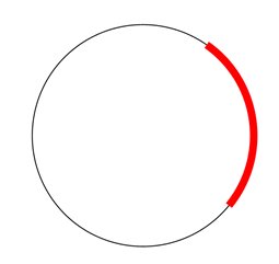
$$L=\frac\times2\pi\, r$$

Truncated Cone

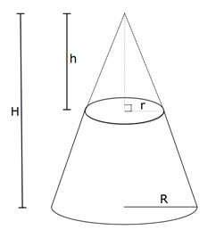
$$V=\frac13\pi(R^2\,H- r^2\,h)$$

$$SA=\pi\,R^2+\pi\,r^2+\pi\,R\,L-\pi\,r\,l$$

Area Sector

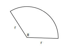
##A=\frac\,\pi r^2##

##L=\frac\times 2\pi r##

Trapezoidal Rule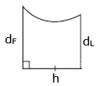

$$A\approx\frac\left\$$

where h is the height of each subinterval

d_F = length of first
d_L = length of last

Electricity

1 KW = 1000 watts

KWH = KW used in an hour

1 joule/second = 1 watt

1 J/s = 1 W

1 kWh = 3.6 MJ

Measurement Error

Error = ±¹/₂ of the smallest division of a scale

Absolute error = ±½ × accuracy/precision

Lower bound = measurement – absolute error

Upper bound = measurement + absolute error

Percentage error = $$\frac\times 100$$

Terminology

¯ Network – collection of objects related in some way to each other

¯ Vertex/Node – point where edges/lines meet, represented as a dot

¯ Edge/Line – line joining the vertices

¯ Loop – line that starts and ends at the same vertex, with no other vertices in between

¯ Degree – the number of edges connected to a vertex

¯ Indegree – the number of edges in a directed network coming in to a vertex

¯ Outdegree – the number of edges in a directed network coming out of a vertex

¯ Directed Network – network where the edges have directions

¯ Planar Network – network with no edges crossing each other

¯ Weighted Network – network where the edges have a number representing time/cost/distance etc

¯ Connected Network – network where all the vertices are connected

¯ Disconnected Network – network where at least one of the vertices are not connected

¯ Walk – sequence of vertices and edges between them
if there are exactly 2 vertices of odd degree, then these vertices must be the start and end
if there are no vertices of odd degree, then the start and end vertex are the same

¯ Closed Walk – walk that starts and ends at same vertex

¯ Path – a walk that doesn’t visit any vertex or edge more than once

¯ Cycle – a path that starts and ends at the same vertex

¯ Trail – walk with no repeated edges

¯ Circuit – a closed trail that starts and ends at the same vertex

¯ Eulerian Trail – trial that includes every edge, no repeated edges – 2 odd vertices

¯ Eulerian Circuit – closed trail that includes every edge, no repeated edges, starts and ends at the same vertex – all vertices even

¯ Hamiltonian Path – visits every vertex only once

¯ Hamiltonian Circuit/Cycle – visits every vertex only once, starting and ending at same vertex

¯ Traversable Graph – trail that includes every edge (without repeating an edge)

¯ Tree – connected network with no cycles (ie only one path between any two vertices)

¯ Spanning Tree – tree that contains all the vertices of the network. (will always have 1 less edge than vertex)

¯ Forest – network with no cycles, and more than one separate spanning tree

¯ Minimum Spanning Tree – spanning tree with the smallest weight

¯ Shortest Path – shortest way in a network

¯ Isomorphic Graph – equivalent graphs (ie same edges and vertices)

¯ Connector Problem – using a minimum spanning tree to find the least cost

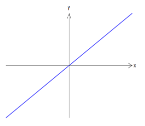
Straight Line

$$y=mx + b$$

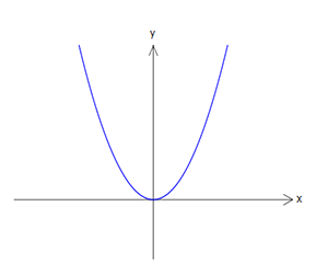
Parabola

$$y=x^2$$

 

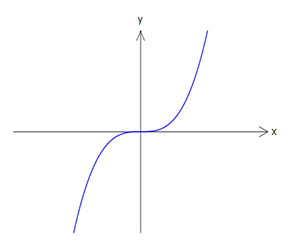
Cubic

$$y=x^3$$

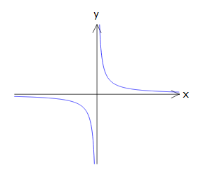
Hyperbola

$$y=\frac1x$$

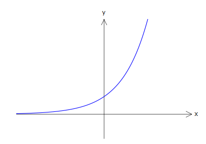
Exponential

$$y=a^x$$

 

Inverse/Indirect Variation/Proportion

$$y \: \alpha \: \frac$$

$$y =\frac$$

where y varies indirectly with x and k is the constant of variation

Terminology

Term	Definition
Range	all probabilities must lie between 0 and 1
Certain	has probability of 1
Even chance	has a probability of ½
Impossible	Impossible
Complementary	events that add to 1

Probability At Least One

P(at least 1) = 1 – P(none)

Two-way Table

•    A positive result means that the test has indicated you have the disease.
•    A negative result means that the test indicated that you do not have the disease.
•    A false positive result means that you have been told you have the disease when you do not.
•    A false negative result means you have been told you do not have the disease when you actually do have it.
•    An accurate positive result means that you have been told you have the disease when you actually do have it.
•    An accurate negative result means that you have been told you do not have the disease when you really don’t have it.

It is VERY important that you read the table carefully, understanding what each cell means. A slight change in the setup can change the interpretation dramatically.

Expected Value & Frequency

Expected Value= The sum of the (probability × outcome)

Expected frequency = probability of event occurring × number of trials

Dice

Capture-Recapture 

Total = original number tagged × total recaptured ÷ number tagged on recapture

Similar Triangles

the scale factor is what you need to times the side in the first triangle to get the number in the second triangle

scale factors can be expressed in two ways

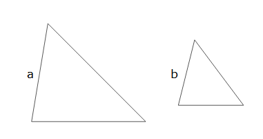
Going from first triangle to second: $$\frac$$

or going from second triangle to first: $$\frac$$

Heart Rate

Maximum Heart Rate (MHR) = 220 – Age in years  beats per minute

Target Heart Rate (THR) is between 65% and 85% of the MHR

bpm = beats per minute

Target heart rate is the desired range of heart rate to ensure the most benefit from a workout

bpm = beats per minute

Target heart rate is the desire range of heart rate to ensure the most benefit from a workout

Data Types

Numerical/Quantitative: quantity/numbers
Discrete – data that can only take exact distinct values – predefined steps
Continuous – data that can take any value

Categorical/Qualitative: categories/words
Ordinal – a natural order is understood e.g. temperature has a natural order: freezing, cold, warm, hot 
Nominal – no natural order is obvious, an order is imposed e.g. favourite colour: red, blue, green – they are in any order

Sampling

Random: each person is equally likely to be chosen, eg, drawn out of a hat

Systematic: some kind of system to select sample, eg, every third person with brown hair

Stratified: same proportion/fraction in the sample as there is in the population

∑	"sigma" means sum ∑f means the total of the Frequency column ∑f(x) means the total of the f(x) column
average	the mean of the scores. To obtain the average, add all the scores and divide by how many scores $$\overline x$$
bivariate data	data wit two variables eg height and weight
cumulative frequency	a total of al the scores before and including the score you are counting now
data	information, scores
frequency	how many of each score there are
fx	the frequency × score
histogram	graph with the bars. Each bar must be the same width, and there must be a gap of half a width at the beginning. The horizontal axis is for scores, the vertical for frequency (or cumulative frequency) and the graph should have a title.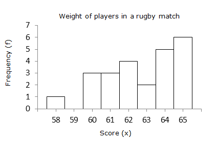
Interquartile Range (IQR)	the middle 50% of the distribution IQR = Q3 – Q1
mean	is also the average. To obtain the mean, add all the scores and divide by how many scores
measures of central tendency	mean, mode, median, range, standard deviation
median	the middle score when they are placed in order
mode	the most frequently occurring, the most common score.
ogive	another name for the cumulative frequency polygon
polygon	line graph, often will go over the top of the histogram.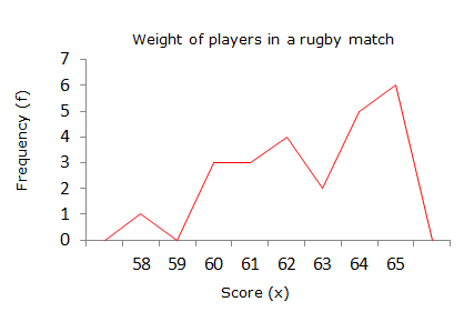
Q1	quartile 1 – the first 25% of the distribution
Q3	quartile 3 – the 75% mark of the distribution
range	the highest score minus the lowest score
score	data
standard deviation	how spread out the scores are
tally	a count of how many of each score there is
$$\overline x$$	"x bar" means average

 

Range

Highest Score – Lowest Score

Mean

$$\bar=\frac$$

$$\bar$$= average

Mode

Most frequently occurring score

Median

Middle Score $$Median=\frac(n+1)$$ score

add 1 to the number of scores and then divide by 2, this will tell you what number score you are looking for

Q₁

$$Q_1=\frac(n+1)$$ score

Q₃

$$Q_3=\frac(n+1)$$ score

Interquartile Range

$$IQR=Q_3-Q_1$$

measures the spread of the middle 50% of the scores

Outliers

Q₁ – 1.5 × IQR
Q₃ + 1.5 × IQR

Z Score

$$z=\frac{x-\bar}$$

x = score $$\bar$$ = average s = standard deviation

Capture Recapture

number originally tagged × number recaptured ÷ number tagged

Line Best Fit

$$y=mx+c$$

$$m=r\frac$$

$$y-intercept = \bar-m\bar$$

Box and Whisker Plots

The box and whisker plot is made up of two 'whiskers' and a box.

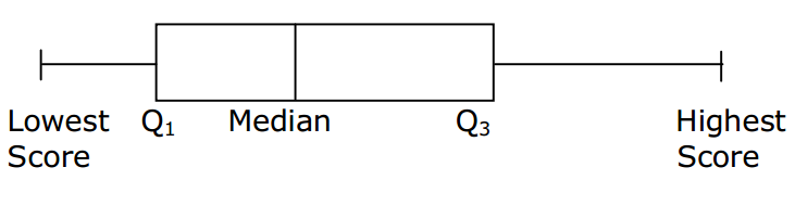
Lowest score: the lowest score in the data set Q₁: the lower quartile, which cuts off the bottom 25% of the scores Median: the middle of the scores, which cuts off the middle 50% of the scores Q₃: the upper quartile, which cuts off the top 25% of the scores Highest score: the highest score in the data set.

IQR

The IQR (inter quartile range) represents the middle 50% of the scores. IQR = Q₃ – Q₁

Outlier

An outlier is a score that is unusual, or different from the bulk of the scores. A score is an outlier if it is more than 1.5 times the IQR (interquartile range) below Q₁ or more than 1.5 times the IRQ above Q_3.

$$z=\frac{x-\bar}$$
$$s=\frac{x-\bar}$$

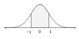
68% will lie between 1 sd above and below the mean

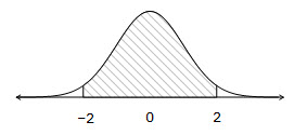
95% will lie between 2 sd above and below the mean

"very probably"

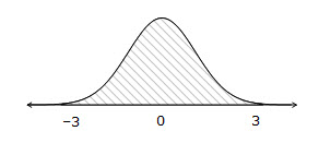
99.7% will lie between 3 sd above and below the mean

"almost certainly"

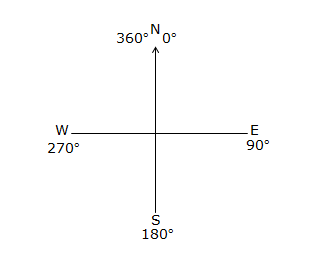
Time

15° = 1 hour

GMT: Greenwich Mean Time

UTC: Universal Coordinated Time (formerly GMT)

DST: Daylight Savings Time: add an hour forward to the time

IDL: The International Date Line

Crossing in an easterly direction, go back a day
Crossing in a westerly direction, go forward a day

Parallels of Latitude

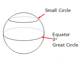
Parallels of latitude are the circles that go around the globe, and a parallel to each other. They are the North or South part.

The equator is in the middle and is 0°.

The Equator is the ONLY great circle of latitude.

Anything above (north) or below (south) the equator is a small circle.
90° North is the North Pole.
90° South is the South Pole.

The radius of the equator is 6400 km.

Small circles have a smaller radius, in relationship to how far away from the equator they are.

Meridians Of Longitude

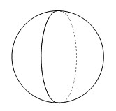
Meridians of longitude go up and down the globe and are the East or West part.

The prime meridian is 0°, and is located at Greenwich (England)

(this is NOT on your formula sheet so learn it!!!)

nautical miles → degrees: ÷ 60
degrees → nautical miles × 60

Spherical Distance

##L=\frac\times 2\pi r##

where θ is the angular distance and r = the radius (6400 for the Earth)

Time Zones

East is ahead in time, the more east, the more ahead.
West is behind in time, the more west, the more behind.

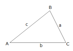
Pythagoras

##c^2=a^2+b^2##

SOH – CAH – TOA

##\sin\theta=\frac##

##\cos\theta=\frac##

##\tan\theta=\frac##

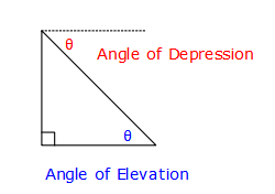
Angles of Elevation & Depression

Sine Rule

##\frac=\frac##

##\frac=\frac##

Cos Rule

##a^2=b^2+c^2-2bc\cos A##

##\cos A=\frac##

Area

##A=\fracab\sin C##

Bearings